甲府市歩行量調査との比較に対する「条件付き混合線形回帰」
PRMLテキスト14章のモデル
https://qiita.com/ctgk/items/3f7e9b37e9bc81b5c063
のプログラム例を修正拡張し甲府市の歩行量調査とWi-Fiデータについての「条件付き混合線形回帰」を試す
2019/07修正(by Namiki)のデータに基づく分析
# ライブラリのインポート
import itertools
import matplotlib.pyplot as plt
import matplotlib
%matplotlib inline
import numpy as np
条件付き混合線形回帰を行う関数の定義
# 計画行列(design matrix)の作成
# 特徴ベクトル(一つのデータ)を1行とし、各データを縦に並べた行列
from functools import reduce
class PolynomialFeatures(object):

    def __init__(self, degree=2):
        assert isinstance(degree, int)
        self.degree = degree

    def transform(self, x):
        if x.ndim == 1:
            x = x[:, None]
        x_t = x.transpose()
        features = [np.ones(len(x))]
        for degree in range(1, self.degree + 1):
            for items in itertools.combinations_with_replacement(x_t, degree):
                features.append(reduce(lambda x, y: x * y, items))
        return np.asarray(features).transpose()
import copy
# 条件付き混合線形回帰の本体
class ConditionalMixtureModel(object):

    def __init__(self, n_models=2):
        # モデルの個数を指定
        self.n_models = n_models

    # 最尤推定を行うメソッド
    def fit(self, X, t, n_iter=100):
        # 推定したいパラメータ(重み係数、混合係数、分散)の初期化
        coef = np.linalg.pinv(X).dot(t)
        self.coef = coef + np.random.normal(size=len(coef))
        for i in range(self.n_models - 1): # バグ修正 (3以上のモデル数に対応)
            self.coef = np.vstack((self.coef,
                                   coef + np.random.normal(size=len(coef))))
        self.coef = self.coef.T
        self.var = np.mean(np.square(X.dot(coef) - t))
        self.weight = np.ones(self.n_models) / self.n_models
        self.rec_coef = [{'step':0, 'coef': copy.deepcopy(self.coef)}]

        # EMステップを指定した回数だけ繰り返す
        for i in range(n_iter):
            # Eステップ 負担率E[z_nk]を各データ、各モデルごとに計算
            self.resp = self._expectation(X, t)
            # Mステップ パラメータについて最大化
            self._maximization(X, t, self.resp)
            # 係数の履歴を記録
            self.rec_coef.append({'step': i+1, 'coef': copy.deepcopy(self.coef)})
    # ガウス関数
    def _gauss(self, x, y):
        return np.exp(-(x - y) ** 2 / (2 * self.var))

    # Eステップ 負担率gamma_nk=E[z_nk]を計算
    def _expectation(self, X, t):
        # PRML式(14.37)
        responsibility = self.weight * self._gauss(X.dot(self.coef), t[:, None])
        responsibility /= np.sum(responsibility, axis=1, keepdims=True)
        return responsibility

    # Mステップ パラメータについて最大化
    def _maximization(self, X, t, resp):
        # PRML式(14.38) 混合係数の計算
        self.weight = np.mean(resp, axis=0)

        for m in range(self.n_models):
            # PRML式(14.42) 各モデルごとに係数を計算
            self.coef[:, m] = np.linalg.inv((X.T * resp[:, m]).dot(X)).dot(X.T * resp[:, m]).dot(t)

        # PRML式(14.44) 分散の計算
        self.var = np.mean(
            np.sum(resp * np.square(t[:, None] - X.dot(self.coef)), axis=1))

    def predict(self, X):
        return X.dot(self.coef)

    def getResponsibility(self):
        return self.resp
# サンプルデータ作成関数 (オリジナル版)
def create_toy_data(sample_size=20, std=0.1):
    x = np.linspace(-1, 1, sample_size)
    y = (x > 0.).astype(np.float) * 2 - 1
    y = x * y
    y += np.random.normal(scale=std, size=sample_size)
    return x, y
# サンプルデータ作成関数 その2 (3種類データ)
def create_toy_data2(sample_size=30, std=0.2):
    x = np.linspace(0, 3, sample_size)
    x = np.hstack((x,np.linspace(0, 3, sample_size)))
    x = np.hstack((x,np.linspace(0, 3, sample_size)))
    y = np.zeros(sample_size*3)
    y[:sample_size] = x[:sample_size] + 0.1
    y[sample_size: sample_size*2] = 2.0* x[sample_size: sample_size*2] -0.5
    y[sample_size*2:] = 3.0 * x[sample_size*2:]
    y += np.random.normal(scale=std, size=sample_size*3)
    return x, y
x,y = create_toy_data2(10)
x
''' 地点の名前を得る '''
import csv
def getPointName(area, kind='name'):
    filename = {"kofu": "/var/www/html/kofu/kofu_position.csv",
               "fuefuki": "/var/www/html/ff/sensor_points.csv",
               "hakushu": "/home/toyoki/public_html/hakushu/points_hakushu.csv"}
    pointName = {}
    with open(filename[area],"r") as f:
        reader = csv.reader(f)
        header = next(reader)
        for line in reader:
            if len(line) < 4:
                continue
            if kind=='group':
                pointName[line[0]] = line[4]
            else:
                pointName[line[0]] = line[3]
    return pointName
データの散布図
# 甲府データの読み込み
import pandas as pd
import seaborn as sns

# テストデータ
df = {}
wifi_data = pd.read_csv('/home/toyoki/work/kofu/reg_analysis201908/wifi_hourly_20181130-20181202.csv')
survey_data = pd.read_csv('/home/toyoki/work/kofu/reg_analysis201908/survey_hourly_20181130-20181202.csv')
df = pd.merge(wifi_data, survey_data, on=['point','date','hour'])
# 地点名
name_of_point = getPointName('kofu')
group_of_point = getPointName('kofu','group')
df['name'] = df['point'].map(name_of_point) # mapには辞書を。または、無名関数を与えてもよい (lambda x: name_of_point[x])
df['group'] = df['point'].map(group_of_point)
# 日にち等の限定 (なければdfそのものを描画)
df4plot = df
#df4plot = df.query('date!="20181130"') # 1130を除外
#df4plot = df.query('date=="20181130"') # 1130だけ
# 描画
sns.pairplot(x_vars=['local_device'], y_vars=['pedestrian'], data=df4plot, hue='name', height=7)

混合線形モデル
負担率を色で表示 (seabornでの表示は今後)
import math
# 学習データの作成
#x_train, y_train = create_toy_data2(std=0.2) # ランダム項の標準偏差=std
# print(y_train)

# kofuデータのデータフレームから混合モデルに合うデータに変換
# 甲府データの利用 (上記で読み込んだものを使う)
x_train = df['local_device'].values
y_train = df['pedestrian'].values

# 特徴ベクトルの定義(次数1)
feature = PolynomialFeatures(degree=1)

# 計画行列への変換
X_train = feature.transform(x_train)
# print(X_train)

# 条件付き混合モデルの用意(モデル数3)
model = ConditionalMixtureModel(n_models=3)

# パラメータの最尤推定を行う
model.fit(X_train, y_train,n_iter=500)

# 結果を図示
x = np.linspace(0, 3000, 200)
X = feature.transform(x)
Y = model.predict(X)
# Figureの初期化
fig = plt.figure(figsize=(12, 8))
# Figure内にAxesを追加()
ax = fig.add_subplot(111) #...2

for i, c in enumerate(model.getResponsibility()): # データ点ごとに負担率(responsibility)で色付け描画
    ax.scatter([x_train[i]], [y_train[i]], color=c)

# 回帰線の描画
ax.plot(x, Y[:, 0])
ax.plot(x, Y[:, 1])
ax.plot(x, Y[:, 2])
std_dev = math.sqrt(model.var)
# 標準偏差の幅で色付けしてみる
ax.fill([x[0],x[0],x[-1],x[-1]],
        [Y[0,0]-std_dev, Y[0,0]+std_dev, Y[-1,0]+std_dev, Y[-1,0]-std_dev], alpha=0.2)
ax.fill([x[0],x[0],x[-1],x[-1]],
        [Y[0,1]-std_dev, Y[0,1]+std_dev, Y[-1,1]+std_dev, Y[-1,1]-std_dev], alpha=0.2)
ax.fill([x[0],x[0],x[-1],x[-1]],
        [Y[0,2]-std_dev, Y[0,2]+std_dev, Y[-1,2]+std_dev, Y[-1,2]-std_dev], alpha=0.2)
plt.show()
print(model.coef) # 回帰係数
print(model.var)  # 分散
# print(model.getResponsibility())

最適化の過程をみてみる
フィッティングの繰り返しごとに回帰係数がどう変化するかを表示
30ステップくらいでほぼ動かなくなる(最適値に達する)ようだ。
むしろ、係数の初期値により結果が異なる、つまり、ローカルな極大が複数あり、初期値によりどの極大値に近づくかが異なる。
coef_data = [] # dataFrameにするために単純な2次元リストにする
for d in model.rec_coef:
    coef = [d['step']]
    coef.extend(d['coef'][0])
    coef.extend(d['coef'][1])
    coef_data.append(coef)
coef_df = pd.DataFrame(coef_data, columns=['step', 'const1', 'const2', 'const3',
                                          'slope1', 'slope2', 'slope3'] )
coef_df.head(20)
# print(model.getResponsibility())
c = model.getResponsibility()
a = np.vstack((x_train, y_train))
#c.shape
a.T.shape
xyc = np.hstack((a.T, c))
# xycが[[x,y,負担率],[],..]の配列になっているかの確認 (上の図と同じならOK)
fig = plt.figure(figsize=(12, 8))
# Figure内にAxesを追加()
ax = fig.add_subplot(111) #...2

for i, c in enumerate(xyc): # データ点ごとに負担率(responsibility)で色付け描画
    ax.scatter([c[0]], [c[1]], color=c[2:])
plt.show()

# 負担率のデータ
point_res_data = pd.DataFrame(xyc, columns=['local_device', 'pedestrian', 'res1', 'res2', 'res3'])
# 元のデータフレームにマージ
df_w_resp = pd.merge(df, point_res_data, on=['local_device','pedestrian'])
df_w_resp.head()
地点の負担率によるグルーピングは可能か
daystr = {'20181130': '金', '20181201': '土', '20181202': '日'}

df_w_resp_1g = df_w_resp.query('date=="20181201"') # ('group=="" and res3 > 0.9') # 一グループ限定
pp = sns.pairplot(x_vars=['res1'], y_vars=['res2'], data=df_w_resp_1g, hue='name', height=6)

#for k,v in df_w_resp_1g.iterrows():
#    # pp.fig.text(v[10],v[11],list(v[9])[0]+","+daystr[str(v['date'])])
#    pp.fig.text(v[12],v[13],v[2]+v[3])

#from IPython.display import display
#display(df_w_resp_1g)

fig, axes = plt.subplots(4, 5, figsize=(15, 12))
plt.subplots_adjust(wspace=0.5, hspace=0.5)
day_color = {"20181130": 'r', "20181201": 'g', "20181202": 'b'}
df_w_resp['color'] = df_w_resp['date'].map(lambda x: day_color[str(x)])
df_w_resp_1g = df_w_resp # df_w_resp.query('date=="20181130"')
for (ax, (key, group)) in zip(axes.flatten(), df_w_resp_1g.groupby('name')):
    ax = group.plot.scatter(x='res1',y='res2',ax=ax, xlim=[0., 1.0], ylim=[0., 1.0], c=group['color'])
    ax.set_title(key, fontsize=8)

計算ごとに、負担率のキー(res1~res3)
次は、曜日ごとのプロット
fig, axes = plt.subplots(4, 5, figsize=(15, 12))
plt.subplots_adjust(wspace=0.5, hspace=0.5)
df_w_resp_1g = df_w_resp.query('date=="20181201"')
for (ax, (key, group)) in zip(axes.flatten(), df_w_resp_1g.groupby('name')):
    ax = group.plot.scatter(x='res1',y='res2',ax=ax, xlim=[0., 1.0], ylim=[0., 1.0])
    ax.set_title(key, fontsize=8)

fig, axes = plt.subplots(4, 5, figsize=(15, 12))
plt.subplots_adjust(wspace=0.5, hspace=0.5)
df_w_resp_1g = df_w_resp.query('date=="20181202"')
for (ax, (key, group)) in zip(axes.flatten(), df_w_resp_1g.groupby('name')):
    ax = group.plot.scatter(x='res1',y='res2',ax=ax, xlim=[0., 1.0], ylim=[0., 1.0])
    ax.set_title(key, fontsize=8)
plt.show()

係数に対する複数の初期値での計算を行ってみる
def mixtureModel4kofu(df, weekend=False):
    # kofuデータのデータフレームから混合モデルに合うデータに変換
    if weekend:
        x_train = df.query('date!="20181130"')['local_device'].values
        y_train = df.query('date!="20181130"')['pedestrian'].values
    else:
        x_train = df['local_device'].values
        y_train = df['pedestrian'].values

    # 特徴ベクトルの定義(次数1)
    feature = PolynomialFeatures(degree=1)

    # 計画行列への変換
    X_train = feature.transform(x_train)

    # 条件付き混合モデルの用意(モデル数3)
    model = ConditionalMixtureModel(n_models=3)

    # パラメータの最尤推定を行う
    model.fit(X_train, y_train, n_iter=500)
    # print(model.coef)  # 回帰係数
    # print(model.var)  # 分散
    return model.var, model.coef


if __name__ == '__main__':
    # テストデータ
    csv_dir = '/home/toyoki/work/kofu/reg_analysis201908/'
    df = {}
    wifi_data = pd.read_csv(csv_dir + 'wifi_hourly_20181130-20181202.csv')
    survey_data = pd.read_csv(csv_dir + 'survey_hourly_20181130-20181202.csv')
    df = pd.merge(wifi_data, survey_data, on=['point', 'date', 'hour'])
    # 地点名
    name_of_point = getPointName('kofu')
    df['name'] = df['point'].map(name_of_point)
    # mapには辞書を。または、無名関数を与えてもよい (lambda x: name_of_point[x])
    coef_list = []
    for i in range(30):
        res_var, res_coef = mixtureModel4kofu(df,weekend=True)
        coef = [res_var]
        coef.extend(res_coef[0])
        coef.extend(res_coef[1])
        # print(coef)
        coef_list.append(coef)
    coef_df = pd.DataFrame(coef_list, columns=['var', 'const1', 'const2', 'const3',
                                          'slope1', 'slope2', 'slope3'])
    from IPython.display import display
    display(coef_df.sort_values(by='var'))
local_deviceとpedestrianの回帰では、分散の最小値は3293であるようだ。これが見た目にももっともよいように見える。
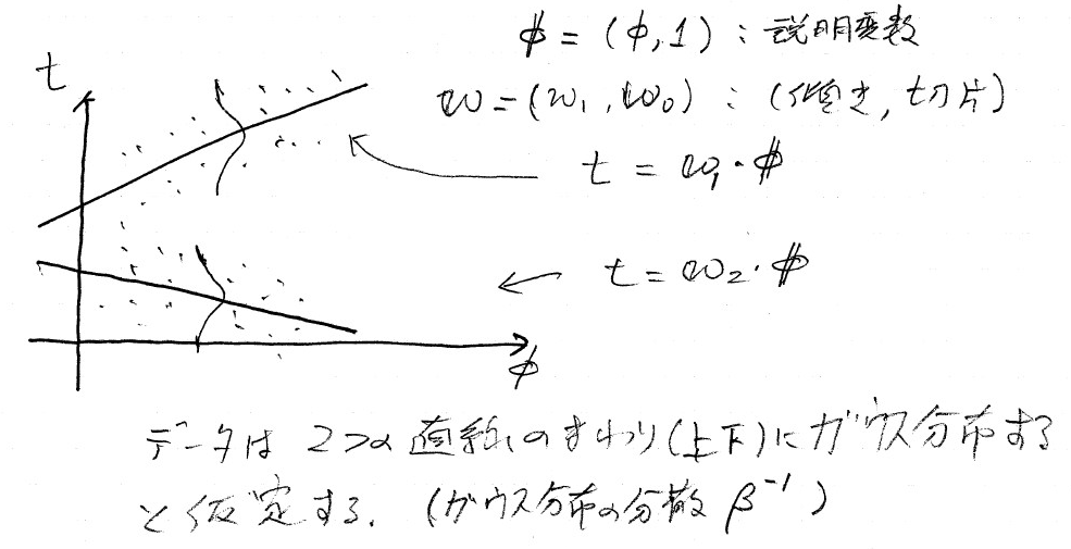
方法についての概念的解説
重み(線形回帰の係数:切片と傾き) ${\bf w}_k$で定義さえる$K$個の線形回帰モデルを考える。データの確率分布は、$K$個の直線の周りにガウス分布すると仮定するのである。
$k$個のモデルの重みを$\pi_k$とし、ガウス分布の分散を$\beta^{-1}$とすると、目的変数の確率分布は $$ p(t|{\bf \theta}) = \sum_1^{k} \pi_k \cal{N}(t| {\bf w}_k^T{\bf \phi}, \beta^{-1}) $$ と書くことができる。$\cal{N}$はガウス分布であり、左辺の${\bf \theta}$は、これから決めるパラメータ${\bf w}_k$、$\pi_k$、$\beta$の総称である。
観測値$\{{\bf \phi}_n, t_n\}$ ($n=1,\cdots, N$) が与えられたときの対数尤度関数(そのようなデータが現れる尤もらしさの対数)は
$$ \ln p({\bf t}|{\bf \theta}) = \sum_{n=1}^{N} \ln \left[ \sum_{k=1}^K \pi_k \cal{N} (t_n | {\bf w}_k^T{\bf \phi}, \beta^{-1}) \right] $$のように表される。
3種のパラメータを、EM法 (Expectation-Maximization method)できめる。EM法は、EステップとMステップの2段階からなり、それを繰り返して尤度が最大になるパラメータを求める。
最初に、上の図の回帰直線の初期値をセットし、データ点に基づいて以下の2段階の最適化を行う。
Eステップ 各データ点の負担率(responsibility)の更新
- 与えられた$\{{\bf w}_k\}$、$\beta$について、各データ点がどちらの直線に近いかの割合(負担率)を決める。
- 負担率を変数として含む対数尤度関数の表式を負担率で微分した式がゼロとなる(つまり極値をとる)条件を解いて「負担率=」の形に表した式。(テキストの(14.37)式)から計算する。
Mステップ 分布のパラメータ${\bf \theta}$を更新する。
- 負担率を固定した対数尤度関数について、それぞれのパラメータで微分した式がゼロとする式を解いて得られる、「パラメータ=」の表式(テキスト(14.38), (14.42), (14.44)式) から計算する。
ここで用いているクラスConditionalMixtureModelでは、この2ステップを繰り返して、最適なパラメータ値を求めている。繰り返しは30ステップくらいで定常値に到達するようである。
最適値を求める式は、対数尤度関数をそれぞれのパラメータで微分した値がゼロになる条件(つまり極値をとる条件)でから導出しているので、グローバルな最大値にはならず、あくまでも局所的な最大値にしか行けない。つまり、一般には初期値に依存してしまう。そこで、初期値を乱数で与え、もっとも良い結果($\beta^{-1}$が小さくなるもの)を与える回帰係数を探す。
詳細
Eステップ
各データについて分担率を決めるために、2値潜在変数${\bf z}_n= \{ z_{n1}, z_{n2}, \cdots , z_{nK}\}$を導入する。$k= 1, \cdots, K$のうちどれか一つだけが$1$となり、他は0である。${\bf Z} = \{{\bf z}_n\}$をパラメータとして含む対数尤度関数は
$$ \ln p({\bf t},{\bf Z}|{\bf \theta}) = \sum_{n=1}^{N} \sum_{k=1}^{K} z_{nk} \ln \left[ \sum_{k=1}^K \pi_k \cal{N} (t_n | {\bf w}_k^T{\bf \phi}, \beta^{-1}) \right] $$初期のパラメータを${\bf \theta}^{{\rm old}}$のもとでの$z_{nk}$の期待値として分担率を求める:
$$ \gamma_{nk} = \mathbb{E}[z_{nk}] = p(k| {\bf \phi}_n, {\bf \theta}^{{\rm old}}) = \frac{\pi_k \cal{N}(t_n| {\bf w}_k^T {\bf \phi}, \beta^{-1})} {\sum_{j} \pi_j \cal{N}(t_n| {\bf w}_k^T{\bf \phi}, \beta^{-1})} $$決定した分担率のもとでの対数尤度の期待値を
$$ Q({\bf \theta}, {\bf \theta}^{{\rm old}}) = \mathbb{E}_{\bf Z} \left[ \ln p ({\bf t}, {\bf Z}| {\bf \theta}) \right] = \sum_{n=1}^N \sum_{k=1}^K \gamma_{nk} \left\{ \ln \pi_{k} + \ln \cal{N}(t_n| {\bf w}_k^{\rm T}{\bf \phi}_n, \beta^{-1} \right\} $$Mステップ
$Q({\bf \theta}, {\bf \theta}^{{\rm old}})$の各パラメータでの微分をゼロとした式より、パラメータ値を求める。